Visualise fields

Setup configuration

Make sure that your simulation.json configuration file has layers.export_field set to true for your desired layers as shown here.

67
68
69
70
71
72
73
74
75
76
77
78
79
80
81
82
83
84
85
86
87
88

    "layers": [
        {
            "name": "F.Cu",
            "file": "F_Cu",
            "type": "copper",
            "thickness": 0.035,
            "export_field": true
        },
        {
            "name": "Dielectric 1",
            "type": "core",
            "thickness": 0.4,
            "epsilon": 4.6,
            "export_field": true
        },
        {
            "name": "B.Cu",
            "file": "B_Cu",
            "type": "copper",
            "thickness": 0.035
        }
    ]

Run simulate with E-field export

gerber2ems --simulate --export-field

Open Paraview

Download and open ParaView from here.

Load E-field data

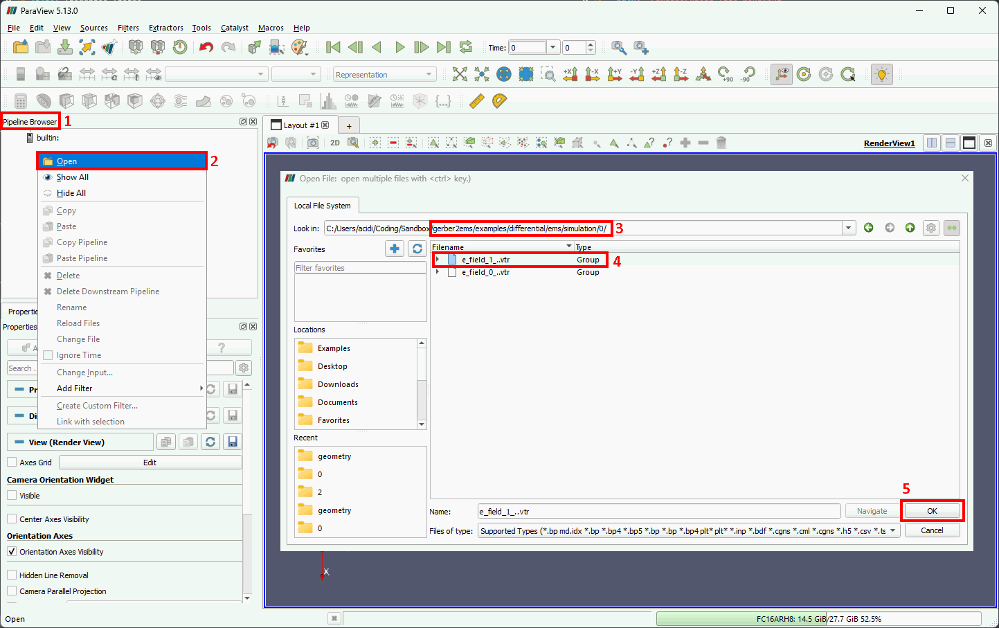
1. Find Pipeline Browser window.
2. Right click inside it and click on Open in the context menu.
3. Navigate to the location of your simulation data.
   • By default it is ems/simulation/{number}
   • {number} is the simulation port index which had an excitation pulse.
4. Select the E-field group data.
   • openEMS generates E-field data in the format of e_field_{index}_{timestep}
   • {index} is the index of the layer in your configuration file which had export_field: true.
   • {timestep} is the timestep in the openEMS simulation when the E-field was recorded.
   • Paraview can load the data as a group for a given {index}.
5. Press Ok to confirm selection.

View E-field data

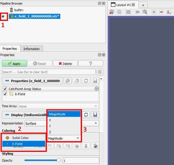
1. Toggle E-field visibility by clicking on the eyeball.
2. In the Properties window under the Coloring section select E-field as your colour source.
3. Select the axis/magnitude of the E-field to view: [Magnitude, X, Y, Z].

Set range to render data

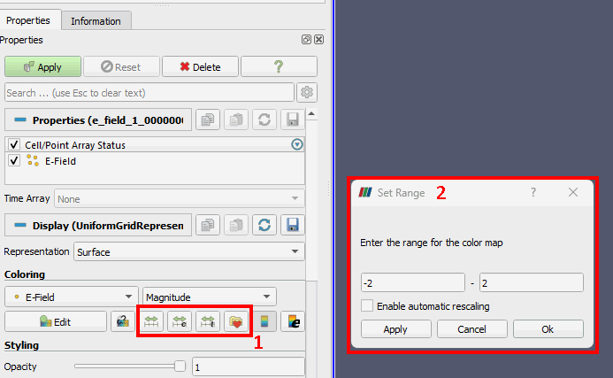
1. There are three buttons to update the visualisation range.

   Method	Use case
   Auto range to current timestep	Visualise data in full range to debug a single time step
   Custom range	Manually set 0 as the centre of the range once minimum and maximum values were found through auto ranging
   Auto range to all timesteps	Reliably visualise the data range across all time steps

2. If scaling manually input values into the dialog box and press Ok to apply new scale values.

Select colour map

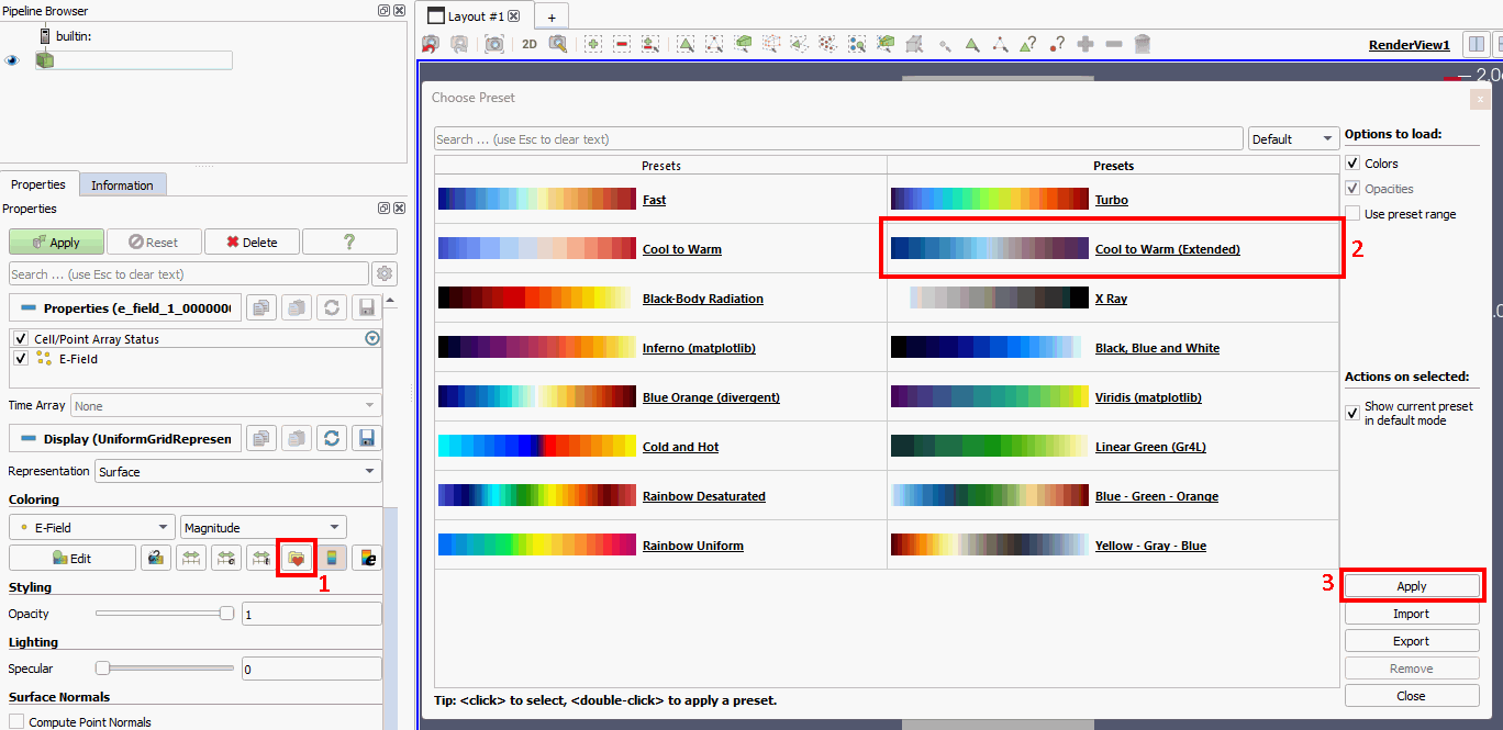
1. Select colour map button.
2. In the colour map presets window select a colour map.
   • If you are visualising the [X,Y,Z] axes choosing a colour map with white in the middle is nicer. This is because the data will contain positive and negative values, where the zero point should be the middle of the colour map (white).
   • If you are visualising the Magnitude selecting a colour map that is zeroed to the lowest value is better.
3. Select Apply to apply colour map.

Playing back timesteps

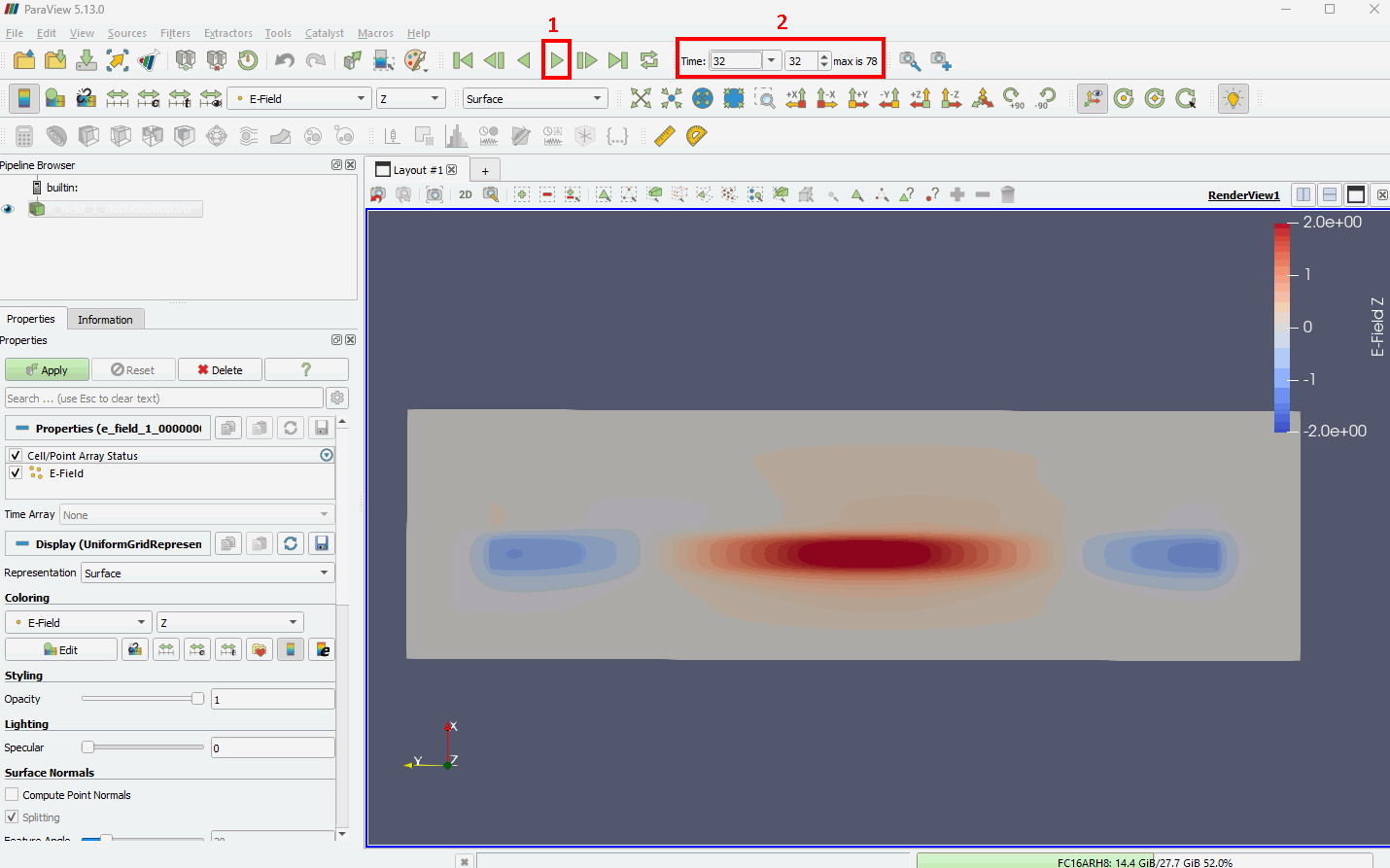
1. Press the play button to begin replaying simulation data.
2. Manually set the time step index to visualise a specific timestep.
3. Go back and update the range if the colours are faded or overblown.

Visualise copper layer

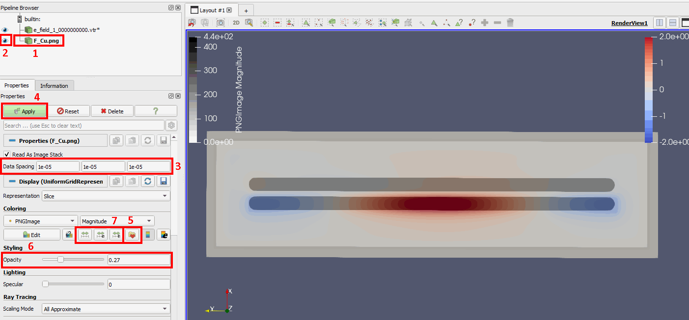
Visualising the copper layer greatly enhances interpretability of E-field data.

1. Load image file of the layer from ems/geometry/*_Cu.png.
2. Enable visibility.
3. Set a data spacing range of 1e-5 to scale image down to size of E-field data.
4. Apply data spacing and visually check if copper layer matches the size of the E-field data.
5. Set the colour map to X-Ray or another colour map that suits you.
6. Reduce the opacity so that the E-field data can be visualised through it.
7. Update the range of the visualisation so that the copper layer appears correctly.